Brain Perfusion Analysis
Having set up your input and output images as described in the Introduction, you can now set up the
quantification parameters for brain perfusion. In the Perfusion
Analysis tool, you will see:
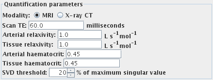
Quantification parameters
First, set the imaging modality by selecting one of:
 if you are working with
Magnetic Resonance Imaging (MRI) data.
 if you are working with
X-ray Computed Tomography (X-ray CT) data.
This determines which quantification parameters should be set.
It is not necessary to set the quantification
parameters if you want semi-quantitative analysis to be
performed. Semi-quantitative analysis will allow you to obtain
relative perfusion parameters, not absolute cerebral blood flow
(CBF) and cerebral blood volume (CBV). However, the mean transit
time (MTT) is truly quantitative regardless of the settings of
these parameters. Regardless of the quantification parameters, the
time-to-peak (TTP) is an assessment of the time to the peak of
contrast concentration, which may be useful for evaluating the delay in
arrival.
Note: it is very difficult to obtain the values you need to
enter for true quantification. These values depend very much on
your pulse sequence and contrast agent, and Xinapse Systems does
not, in general, recommend that you try to obtain quantitative
perfusion parameters.
Now set the following parameters, if applicable:
- Scan TE (MRI data only). The scan is assumed to be T2 or
T2*-weighted. For quantification, enter the correct
echo time.
- Arterial relaxivity (relaxivity of the contrast agent
for large vessels) (MRI data only). This is the slope of the plot of
R2* versus concentration of contrast agent in
the blood plasma in the large vessels. Needed
for quantification, otherwise leave as 1.0.
- Tissue relaxivity (relaxivity of the contrast agent for
the capillary bed) (MRI data only). This is the slope of the plot of
R2* versus concentration of contrast agent in
the blood plasma in the capillaries. Needed
for quantification, otherwise leave as 1.0.
- Arterial haematocrit. The haematocrit in large vessels. Needed
for quantification, otherwise leave as 0.45.
- Tissue haematocrit. The haematocrit in the capillary bed. Needed
for quantification, otherwise leave as 0.45.
- SVD threshold. This affects the sensitivity of the analysis to
noise and pseudo-random variation in the input images. Increasing
this value will make the analysis more immune to noise, at the
expense of bias in the quantification. The default of 40% should
be fine for most images.
Arterial Input Function (AIF)
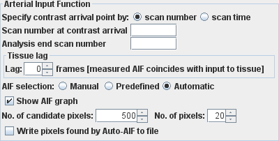
To obtain an arterial input function (the concentration of
contrast agent in an artery that feeds the brain), you must set
the following:
- The time at which contrast agent first appears in the feeding
artery. If you cannot see a feeding artery and are obtaining the AIF
by some other means, then this should be the time at
which the image first changes in intensity as the contrast arrives in the
tissue. By selecting from
 , you can
specify this either as:
- The time at which contrast first appears (the first
image is acquired at t=0).
- The scan number at which contrast first appears (the first
scan is numbered 1).
Enter one of these. You can graphically confirm the arrival time using the
Roaming Response dialog.
- You may optionally enter the time at which the series of images is truncated
for the purposes of analysis using
 .
Images after this time will not be used as part of dataset for the analysis. Analysis will
proceed as if the data after this time point has not been acquired.
By selecting from
 ,
you can specify this either as:
- The time at which to truncate the data set, or
- The scan number at which to truncate the data set.
Enter one of these, or leave the field blank to use the whole dataset.
You can graphically confirm the time of truncation using the
Roaming Response dialog.
- Any lag from the measured arterial input function to the
actual arterial input feeding directly into the tissue. This is specified as a
number of frames (time points) of lag. Change the AIF lag using the AIF lag spinner.

The text to the right of the spinner explains the meaning of the lag value you set.
- Choose how you want to obtain the AIF. You can:
- Manually draw round one or more feeding arteries to produce a
set of regions of interest (ROIs). In this
case you can produce an ROI file that contains one or more ROIs drawn
at one particular time point. This same set of ROIs will be used for
all time points to obtain the AIF. Alternatively, you can define a set of ROIs at
one time point, then copy and paste them to the same slice location for all time
points, and manually adjust the position to account for patient movement
during the scan. If you do this, the tool will expect to find a set of ROIs at
every time point, and will given an error if it does not.
Select the ROI file used for the AIF by pressing the
 button, or
type the name into the text field:

- Use a predefined AIF. You can read the values of the AIF from
a file that contains a list of concentration of contrast
agent values. The file must contain two columns of numbers:
- The first column is the time at which the concentration of contrast agent ([Gd])
is measured.
- The second column contains the blood plasma concentration values (moles/L).
Whitespace or a comma (",") should separate the two columns.
Note: the format required for the AIF file has changed between Version 6 of and Version
7 of Jim. The first column (time values) is now used. The onset of the arterial input
function is taken to occur at the first time point where the concentration value first rises
above zero. This time point (after taking account of any tissue lag that you input) is taken to
co-incide with the time that you specify for contrast arrival. The time between measures of
the concentration may now be unevenly-spaced and does not have to match that of the input
images. The pre-defined AIF is automatically resampled to the required time-base of the input
images.
The Perfusion tool will output such a file for every analysis it
performs, which will give you an example of what is needed. For
semi-quantitative analysis you just need values that are
proportional to the concentration of contrast agent in
the artery.
Select the file used for the predefined AIF by pressing the
 button, or type the name into the text field:

- Automatic AIF finding - Jim finds the pixels that have AIF-like
characteristics. Note: this option is not available for X-ray CT images.
- First, Jim makes as sweep of the whole image and selects pixels that
have a the largest intensity change. The number of pixels selected is set
in the "No. of candidate pixels" spinner.

Typically this would be set to around 1% to 5% of the total number of
pixels in the image. Setting a smaller number here will speed up finding
of the AIF, but may cause the tool not to select the best AIF pixels.
- Next, these candidate pixels are searched for pixels that
have the most AIF-like characteristics. The final number of pixels used to define
the AIF is set in the "No. of pixels" spinner.

AIF-like characteristics are: a large transient signal change occurring shortly
after contrast injection.
You can visualise the pixels that are have been found by auto-AIF by selecting:

Each pixel found is outlined by a Rectangular ROI and written to an ROI
file. The name of the ROI file is constructed from the output image base
name that you set, with the suffix AutoAIF.roi.
- Check the "Show AIF graph" check-box if you would like a window
to pop up showing you the AIF that is being used in the perfusion analysis.
Brain Perfusion Output Parametric Images
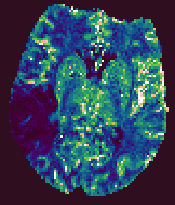
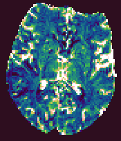
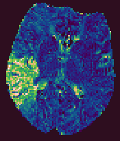
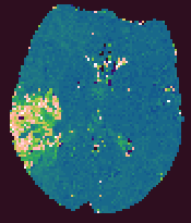
The Brain Perfusion analysis produces five output images, that
have the same base name, but have the output parameter name
appended. These are:
- CBF. Cerebral blood flow, with units of mls blood / 100g tissue / minute.
- CBV. Cerebral blood volume, with units that indicate the blood
volume as a percentage of the total tissue volume.
- MTT. The mean transit time, in seconds.
- TTP. The time from contrast arrival to the peak in capillary concentration, in seconds.
- RMSE. A measure of the goodness of fit. This root-mean-square of the residuals between the
fitted curve and the time-series data.
These output images are in floating-point format, and can be
viewed using Jim. The output images will be of the same
image type as the first input image.
Example output images from the Brain Perfusion Tool.
 |
 |
 |
 |
| Cerebral Blood Flow |
Cerebral Blood Volume |
Mean Transit Time |
Time-to-Peak |
What Happens When Fitting Fails?
Perfusion analysis failure may be caused by several factors:
- The data are too noisy to perform an accurate fit.
- The data are corrupted by artefacts.
- The model is a poor match to the data.
Any pixel
where perfusion analysis fails will have a value in all output images which is either
zero, or NaN (not-a-number). Which of these two is written to the images is controlled by a
setting in the user preferences.


 if you are working with
Magnetic Resonance Imaging (MRI) data.
 if you are working with
X-ray Computed Tomography (X-ray CT) data.

 , you can
specify this either as:
 .
Images after this time will not be used as part of dataset for the analysis. Analysis will
proceed as if the data after this time point has not been acquired.
By selecting from
 ,
you can specify this either as:

 button, or
type the name into the text field:

 button, or type the name into the text field:


![]()

